Abridged notes on the LLM scaling book

Essays on ML systems, looking at LLMs on TPUs

In February, folks at Google DeepMind published a book on LLM scaling.

The book focuses on how you can model LLM scaling with math. I’m a big fan of stuff like this. Intuitive reasoning about systems is really important; it lets you visualize their shape and behaviors at a glance.

How to Scale Your Model (2025)

I thought it would be a good time to read, learn and add some personal commentary (as someone working in the industry at Modal). Expect these notes to be super abridged and not a book replacement — I will skip things, and any errors are my fault.

(I’m still working on jax-js, by the way. It’s going well! Since the last update in May, 3 months ago, we’ve went from matrix multiplication to full neural networks, complex operations like softmax + convolution, optimizers, and kernel tuning / optimization. The project is now over 10,000 lines of code.)

Without further ado, let’s begin!

Part 0: Intro

This book is about scaling LLMs on TPUs. In the past, ML researchers didn’t think so much about performance. But today, research takes a lot of compute.

ML systems are complex enough that you can’t just fiddle with parameters until they becomes fast. You need a deep understanding of how long it takes to run LLMs, based on compute, memory, and network factors. This informs the fundamental research you do, as well as systems design and efficiency.

We’ll then discuss:

• Transformer architecture, FLOP math for forward and backward passes.

• Parallelism strategies (data, tensor, pipeline, expert) and other tricks (FSDP, host offload, gradient accumulation) for scaling LLM training and inference with increased numbers of GPUs and nodes, hopefully linear in performance.

• Practical examples in JAX and with the LLaMA-3 model.

• The final chapter is about Nvidia GPUs.

Part 1: Rooflines

The roofline model considers communication time and computation time:

(Note: Communication could either be a single chip, loading from global memory in a GPU, or multi-chip / multi-node links like PCIe, NVLink, Infiniband, RoCEv2, …)

\(\max(T_\text{math}, T_\text{comms}) \leq T \leq T_\text{math} + T_\text{comms}.\)

Typically, we use the maximum of communication and computation, since you can overlap them in most cases. But even if you can’t overlap them, it’s a good approximation, since it’s off by at most a factor of 2.

Since there’s a max() here, we have two regimes:

• Compute-bound: T_math > T_comms. You are getting full utilization from your hardware, and the link is not saturated.

• Comms-bound: T_comms > T_math. You’re wasting at least some of the FLOPs/s from your hardware, waiting on the saturated link.

You want to be compute-bound, since that’s what you’re paying for — FLOPs.

Assuming a well-written kernel, you can estimate whether it will be compute-bound based on the arithmetic intensity AI = W/Q, or work over memory traffic. On TPU v5e MXU, you want ≥240 FLOPs/byte for bfloat16 (= compute / mem bandwidth).

For matmul in neural networks, this translates to a batch size of ~240 (0.5*AI for bfloat16 = 2 bytes, but 2*AI because of 2 FLOPs).

You can do the same roofline analysis for tensor parallelism: splitting along the reduction axis in a neural network. This would give us a critical threshold in the rough thousands for reduction axis length when this is viable (basically: each device needs to do at least X work per byte transferred).

Roofline analysis is the main way to evaluate parallelism.

Part 2: How to Think About TPUs

TPUs are tensor cores on high-bandwidth memory (HBM). They can do matrix multiplications fast with systolic arrays. Lots of FLOPs for matmuls.

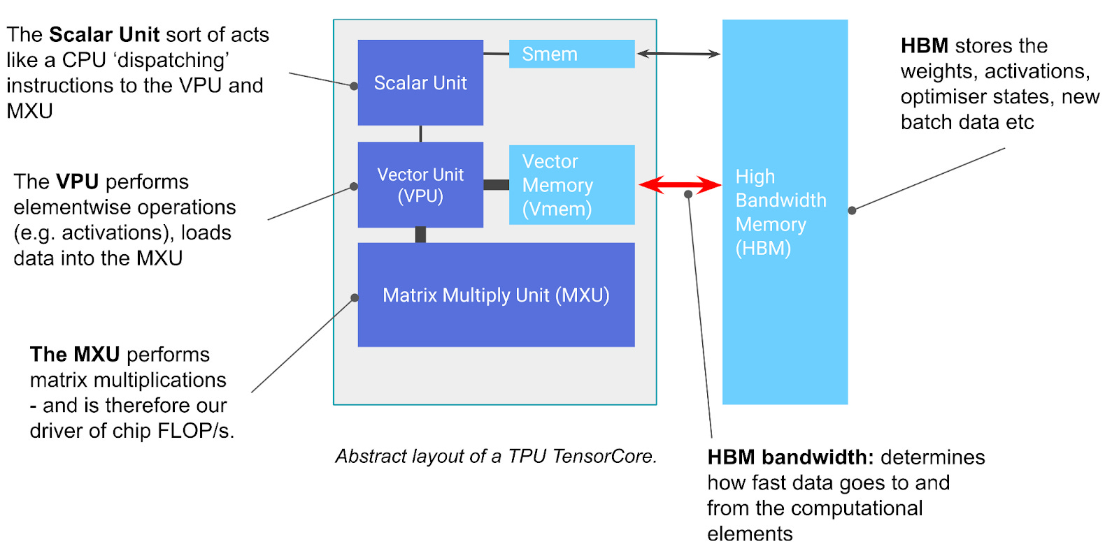
How does it work? There are some animations about the pipelining and systolic array architecture on the hardware level. Basically, it does a 8x128 x 128x128 → 8x128 matmul every 8 cycles, and it’s very fast but needs a bit of ramp-up.

There are two kinds of memory on a TPU chip (1 chip = 2 cores, shared HBM):

• HBM is the main memory, similar to GPUs. This is ~16-95 GB, ~1 Tbps.

• VMEM is smaller working memory / cache. It’s about 0.1 GB, much smaller but tops out at around an intensity of about 10-20 FLOPs/byte. Good for fast inference on small-batch workloads if you can fit weights.

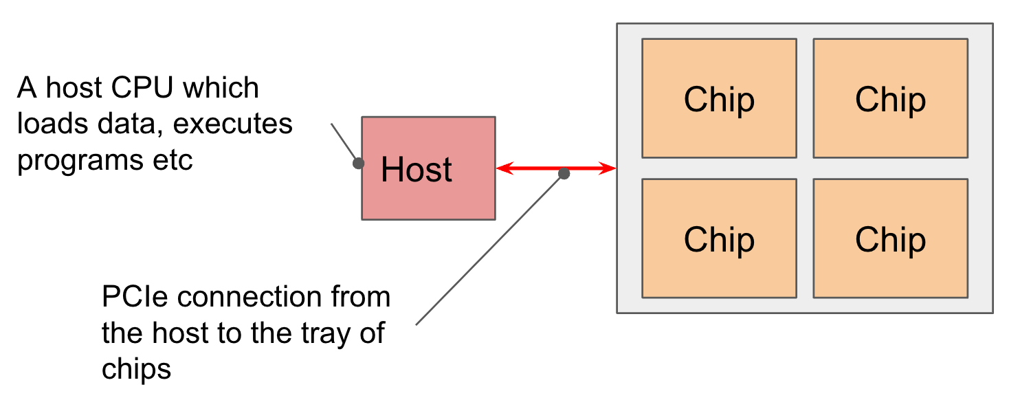
Chips are “logical megacores” each consisting of two cores. Four chips are exposed on a single TPU-VM host with PCIe (~200 Gbps NIC).

TPUs are connected to each other in 2D/3D torus configurations with ICI, inter-chip interconnects. These are ~1.6-4.8 Tbps, and there 4 or 6 of them. Compare to Nvidia’s 3.2 Tbps Infiniband cluster networking.

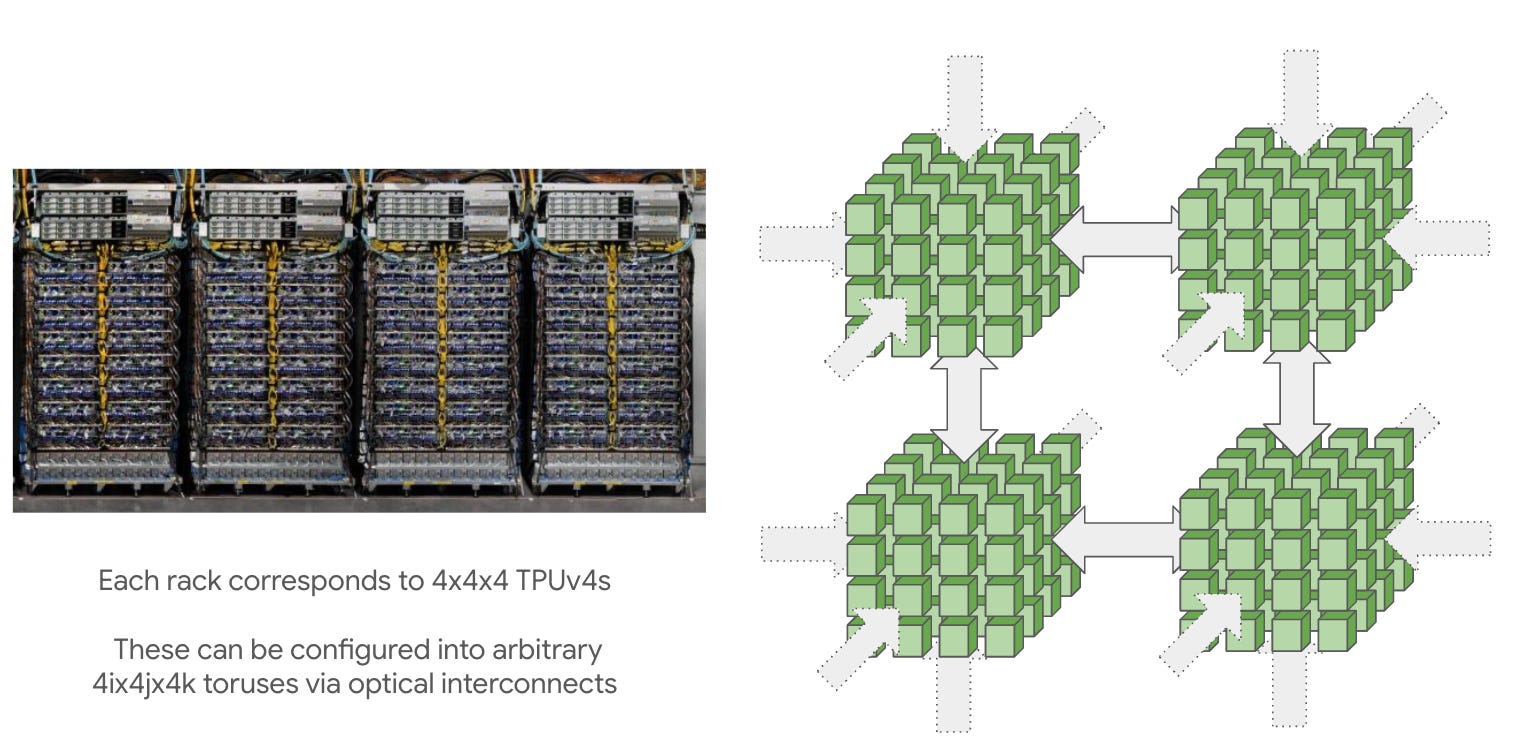
It’s cheaper and more scalable than fat tree-style networks that Nvidia uses for Infiniband, but it probably makes collective communication tricky. When you purchase TPUs from Google, you buy a slice of the topology.

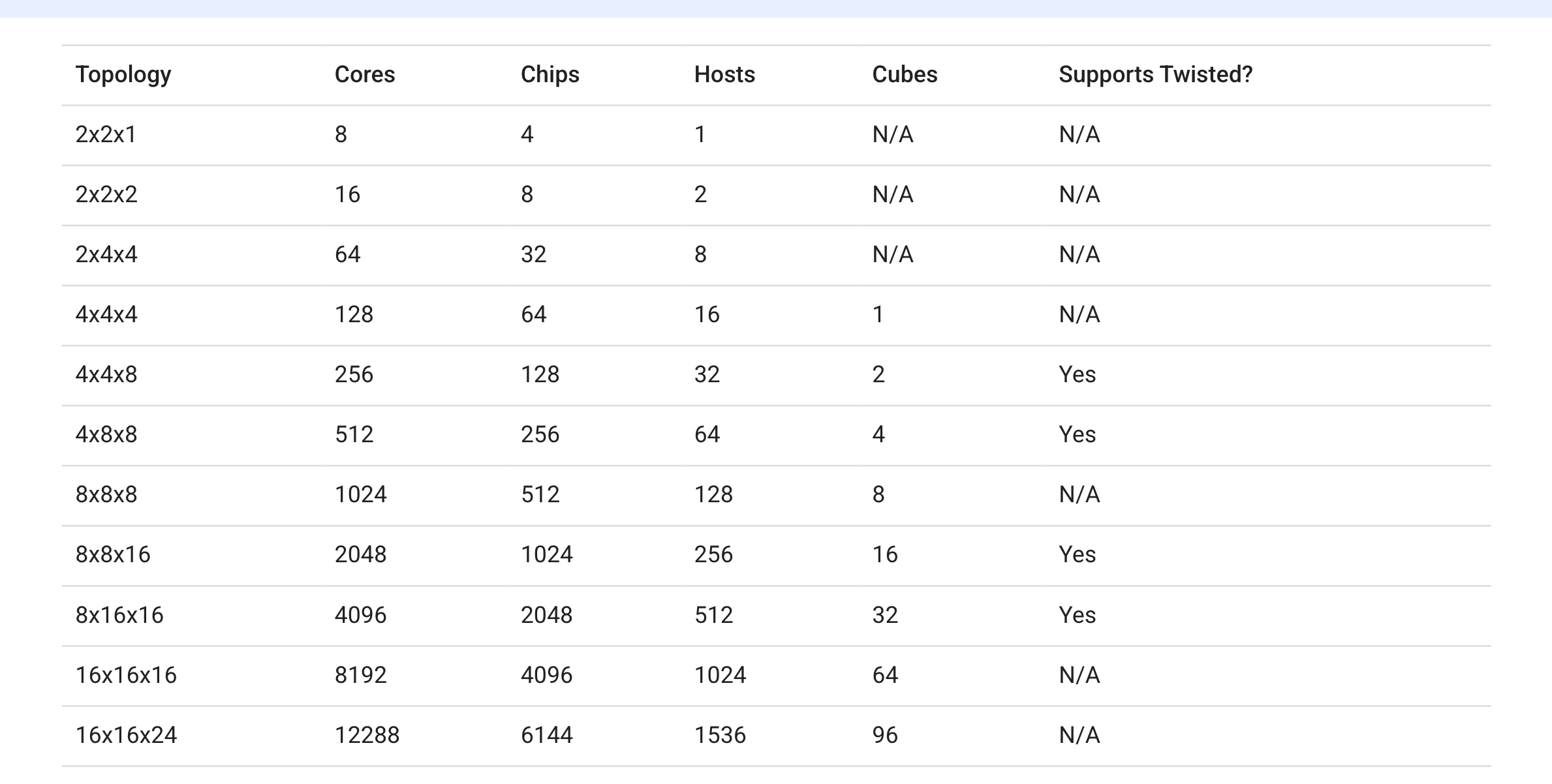
The smallest slice is a single 2x2x1 host. This checks out with each host being connected to 4 TPU chips.

Part 3: Sharded Matrices and How to Multiply Them

We introduce tensor notation for device sharding. When you have multiple devices (relevant for TPUs especially due to topology), they live on a mesh with axis names. For example, a 2x2 mesh of 4 TPUs, with axes (X, Y):

Mesh(devices=((0, 1), (2, 3)), axis_names=(‘X', ‘Y'))

Notation for sharding arrays is A[Ix, Jy]. The indices can be subscripted by mesh axes, which tells us how each mesh axis corresponds to a tensor axis.

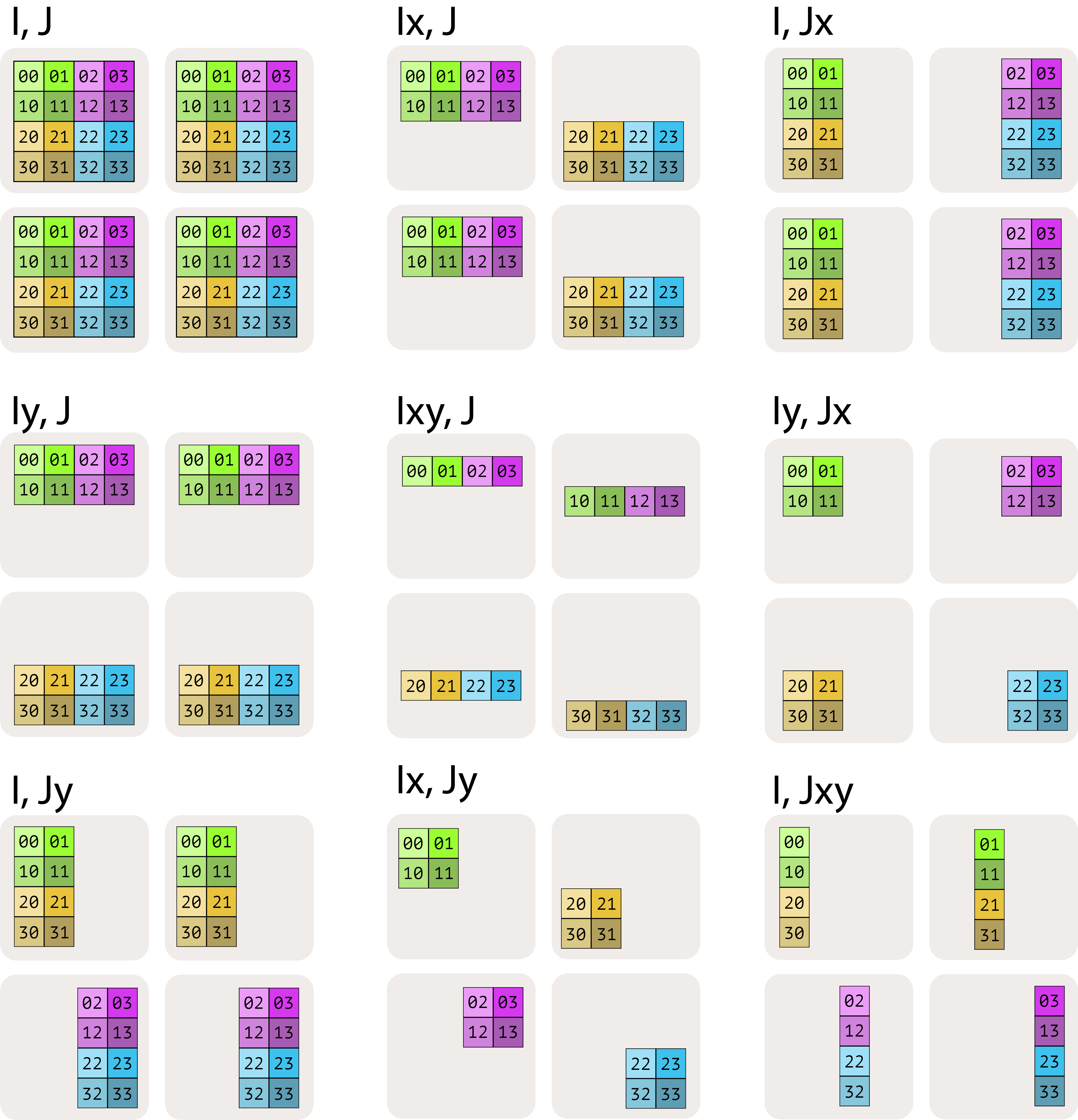
There are a couple rules to this notation system. Internalizing the rules will help you reason about device sharding:

• Not all mesh axes need to be mentioned in a sharding. For example, A[I, J] would fully replicate the array across all axes. A[Ix, J] would shard the first tensor axis against X and replicate the rest along Y.

• Each mesh axis can be mentioned at most once. A[Ix, Jx] is invalid, since that doesn’t actually include all the data.

• The order of axes matters. A[Ixy, J] shards the first tensor axis on both dimensions of the mesh. But it shards against the X mesh axis first, and then the Y mesh axis second. Contrast this with A[Iyx, J], which reverses the order.

This notation lets us talk about tensor sharding over TPU devices in a torus. Each mesh axis and can do full collective operations like AllReduce, AllGather, and ReduceScatter. Next, we ask the big question.

Question: How long does it take to do matmul on sharded arrays?

Matrix multiplication is a tensor contraction (“like numpy.dot”) op. When you do a dot product of A[I, J] * B[J, K] → C[I, K], you’re contracting along the J axis.

Generally, if your tensor is sharded along the contracting dimension, you may need to use one of the collective operations:

1. Case 1: neither input is sharded along the contracting dimension. We can multiply local shards without any communication.

2. Case 2: one input has a sharded contracting dimension. We typically “AllGather” the sharded input along the contracting dimension.

3. Case 3: both inputs are sharded along the contracting dimension. We can multiply the local shards, then “AllReduce” the result.

4. Case 4: both inputs have a non-contracting dimension sharded along the same axis. We cannot proceed without AllGathering one of the two inputs first.

I think Case 3 is probably the most illustrative one, since it’s the AllReduce that you typically see when you shard computations along a contracting dimension and need to aggregate the results.

They have derivations to work through and very nice animations. Here’s a summary of the communication primitives and their effect:

• AllGather: [Ix, J] → [I, J]. Costs |I|*|J| comms/device.

• ReduceScatter: [I, J]{Ux} → [I, Jx]. Costs |I|*|J| comms/device.

• AllToAll: [I, Jx] → [Ix, J]. Costs 0.5*|I|*|J| comms/device (assuming 2D torus).

• AllReduce: [Ix, J]{Uy} → [Ix, J]. Costs 2*|I|*|J| comms/device.

  • This is the same as ReduceScatter + AllGather.

Notably, the AllToAll primitive is suited for toroidal TPU topologies. The other collective operations use a standard ring algorithm.

Part 4: All the Transformer Math You Need to Know

We start with some tensor math. When you have a dot product, some axes are contracting, some are batching, and others are just broadcast. Cheatsheet:

• Contracting: I * I → ∅. This is a reduction axis.

• Batching: I * I → I. This axis is mapped / vectorized over in both tensors.

• Others: I * J → IJ. The axes are broadcast like an outer product.

The total number of FLOPs equals 2x the product of all axes, taking care not to double-count them if they appear in both operands of the product.

The reverse pass (backprop) takes twice the number of FLOPs as the forward pass. This isn’t exactly the case for all operations (i.e., scalar ones), but since most FLOPs in a transformer are in matmuls, a good rule-of-thumb is to multiply the total FLOPs by 3 (= 1 + 2) when thinking about training.

Anyway, if you go ahead and use this trick, you get all the transformer FLOPs.

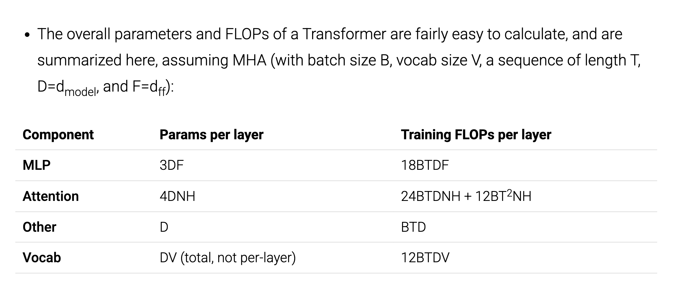
Or, in a nutshell: multiply params by 6BT (BT = #tokens), and some of the multi-head attention layers scale by 3BT²/D instead.

Great! Will be useful for thinking about KV cache later, too.

Part 5: How to Parallelize a Transformer for Training

This chapter is about train-time scaling. Assume big but fixed batch size (too big slows down convergence), so you’re compute-bound on the chip itself for HBM access. You want to use more chips to speed up each iteration.

My tl;dr is that you can scale things along different axes: data parallelism (or FSDP), tensor parallelism, and pipeline parallelism. These are along different axes: batch, model, and layers. Each of them stresses a different communication overhead, so if you combine all of them together, you can coordinate very low batch sizes per device without being comms-bound! (i.e., run lots of devices, train fast)

That means there’s no “best” parallelism strategy. You apply all of them as needed, since they multiply together. Start with data parallelism though (it’s easy).

I’m going to ignore the TPU numbers here and speak more generally, since I only use GPUs in my job anyway. The TPU numbers are kind of messed up versus GPUs because of the bandwidth (here, in-and-out):

• TPUs have more ICI bandwidth (v5p = 4 * 0.8 Tbps / v5e = 6 * 2.4 Tbps) in bigger “pods” of up to 8960 chips, but wide-diameter torus connectivity, and

• GPUs have NVLink (7.2 Tbps, fully-connected) within nodes of 8 GPUs each and Infiniband (0.125 * 3.2 Tbps, switched tree) connections between nodes. Also, each GPU has more FLOPs than each TPU.

This means TPU clusters can skip pipeline parallelism, which is complicated, but GPU clusters need to use it for inter-node to reduce comms overhead.

Data parallelism

This is the simplest method.

1. Split the batch across X devices and do the forward and backward passes independently.

2. (Interleaved) When gradients are ready for a layer, do an all-reduce, then update optimizer state with the accumulated gradients across all devices.

You become bottlenecked on comms when B/X > C/W_ici. In other words, the number of FLOPs divided by the bandwidth. (The constants cancel out for fp16.)

Within an 8x H100 node, data parallelism takes (1979 TFLOPs) / (900 GB/s) ~ 2200 required batch size per GPU to max out compute with sparsity, or ~1100 without.

But between nodes, your bandwidth per GPU is 18x lower. So you’d probably want to run ReduceScatter first between GPUs within each node, followed by AllReduce inter-node (8x less comms) and another AllGather within each node.

FSDP / ZeRO-3

Ah yes, the famous fully-sharded data parallelism. It’s like DDP, but model weights & optimizer states are sharded. Each device stores 1/X of the params. See the “experiences” FSDP paper for details on this, including how to interleave compute and comms within the framework.

Compared to DDP, you incur 1.5x comms cost in mixed-precision training (“full sharding” at least, they also have “hybrid sharding” which is partial DDP), since you have to AllGather weights in addition to the AllReduce of gradients.

It’s said that the FSDP backward pass is “free” though, in the sense that you shard optimizer state and weights with AllGather+ReduceScatter, while reducing FLOPs. This is also the difference between ZeRO-1, ZeRO-2, and ZeRO-3 = FSDP.

FSDP lets you scale up model sizes that don’t fit in a single GPU’s memory.

Tensor parallelism (Megatron)

Let’s switch our mesh axis from X to Y. Tensor parallelism shards both the weights & activations across devices. It makes each layer run faster because we don’t have to do as much work on each device, but we do need to insert AllGather / ReduceScatter ops in the forward and reverse passes.

Generally, this becomes worth it when the dimension of the MLP hidden layer exceeds C/W_ici * Y.

In other words, you can start splitting apart the model with tensor parallelism on H100 GPUs if the model dimension is over ~250 or so (since there’s 4x expansion ratio). This becomes very useful for large models, and it combines well with FSDP. Generally the tensor parallel factor is 8 or 16.

Pipeline parallelism

The book doesn’t really talk about pipeline parallelism since it’s mostly used on GPUs. It saves comms overhead by only requiring you to transfer activations between layers, while also partitioning the model and speeding up training. This way, you don’t actually have to send O(weights) data, only O(activations).

The hard thing here is avoiding bubbles. Honestly pipeline schedules make my head hurt. But people have figured it out, likely at great engineering cost!

Takeaways

With enough parallelism strategies, we can achieve near-linear scaling over many nodes while keeping batch size per device low, nearing ~100. Each choice requires a lot of engineering effort though, especially for interleaving operations and reliability in the face of failures.

You can combine the strategies together (DP+TP+PP) for multiplicative bonus. Requires you to do some math though.

Part 6: Training LLaMA 3 on TPUs

This was just an applied exercise of the previous section.

One interesting thing was that they introduced “sequence parallelism” here, which is similar to data parallelism but over the sequence axis. This happened when they ran out of “batch” to FSDP over. I guess this introduces a bit more comms overhead, but not too much since you’re just syncing activations ahead of attention.

I was also curious about the cost for this hypothetical training of LLaMA 3 70B with 40% MFU on TPUs. Assuming 3-year commitment prices, you get:

8960 chips * $1.89/chip/hr * 1056 hours = $18 million

That’s just a 70B model. Makes sense why the big labs are raising billions of dollars for their frontier models with trillions of parameters.

Part 7: All About Transformer Inference

Inference is very different from training. You have a latency-throughput tradeoff curve, since big batches take longer but vastly improve throughput due to higher arithmetic intensity, being less memory-bound.

(This section is also relevant in post-training, since you do rollouts for RL.)

Basics of transformer inference

Alright, as we know: to sample from a transformer, you run prior tokens through the model layers. This generates logits, you draw from the posterior according to temperature, and then you repeat the process again for each subsequent token.

You also need a paged KV cache though, so you don’t need to recompute intermediate activations each time. Instead, you reuse the previous ones. KV cache size is proportional to the sequence length, number of layers (L), number of KV heads, and model dimension (D), Example: flash_attn_with_kvcache().

Given this KV cache, there are two phases to inference:

1. Prefill. Generate all the KV cache for a long prompt, and generate first set of logits. Initializes the cache.

2. Generation (also “decode”). From a previous KV cache for all previous tokens in the sequence, incrementally sample one token and generate logits. Appends +1 token to cache.

Although, engines like vLLM can run both simultaneously (“chunked prefill”), and perhaps other inference systems may also split across separate machines (“disaggregated prefill”).

Anyway, here’s the tl;dr about the two parts of inference from a performance lens:

• MLP: Arithmetic intensity. Token batch size ≥ FLOPs / HBM bandwidth.

  • For TPU v5e, ~240. For H100, this is ~600 (with sparsity) or ~300 (without).

  • Critical batch size decreases with param quantization (less loads), but increases if FLOPs are in lower precision since they become faster.

  • Trivial to get this batch size in prefill with sequence length, harder during inference to batch up many concurrent requests.

• Attention: With S past tokens and T inference, AI ~ ST / (S+T).

  • During prefill, with cross-attention you get a good arithmetic intensity, linear with batch size, easy to saturate and not the bottleneck.

  • During decode, AI ~ 1 because you load all of the weights from KV cache. You’re bottlenecked on memory bandwidth, loading from KV cache, since each of those is only used once in attention.

  • So yeah, that’s sad. Once you increase your decode batch size enough, you’ll get diminishing returns — each forward pass gets slower because loading memory from KV cache dominates model weights size.

This observation about the memory-bound nature of attention is fundamentally why we have a latency-bandwidth tradeoff. You can’t actually run transformer inference (decode) at the MLP critical batch size of ~300, without sacrificing lots of time on loading KV cache, slowing down inference (inter-token latency).

If you squint a bit, this is also the graph you get when benchmarking vLLM / SGLang.

Tricks to improve latency / throughput

At scale, we do actually want to run big batch sizes and not waste all our time on memory bandwidth to load the KV cache! It would also be nice to make the KV cache smaller on a per-token basis, since that saves memory. So we have two, mutually beneficial reasons to reduce KV cache.

Here are common tricks people do in service of this goal:

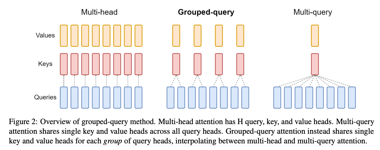
• Grouped Query Attention (GQA) reduces the number of KV heads and shares each with multiple Q heads. You can pick along a sliding scale between 1 KV head per Q head (standard multi-head attention), up to just 1 KV head in total. Seems like not all of the KV heads are needed for performance!

  

• Mixing local attention layers is done by some models. For example, Gemma 3 uses 5 local layers between each global attention layer. GPT-OSS alternates between local and global attention in a 1:1 ratio. The idea is that you can focus on local details most of the time, and this reduces KV cache.

• Sharing KVs across layers: You can go even further than GQA and share the KV’s across layers, not just queries. It reduces KV cache size, but it doesn’t reduce memory bandwidth since they need to be read in each layer.

• Quantization saves on memory bandwidth and size for both params and KV cache. If you keep activations at the same precision, it helps reach the roofline.

• Paged attention uses ragged reads into sections (“pages”) of HBM that are allocated as needed, based on the sequence length. It adds a bunch of complexity around memory allocation, preemption and interleaving, but it’s used by almost every inference engine to save memory. See nano-vllm’s scheduler.

Distributing inference

If you’re scaling to multiple accelerators, now you have the opportunity to explore various parallelism strategies. The default is to just replicate the model, with all of its weights in multiple instances, which is simple and doesn’t need any comms / syncing.

But you might want to speed up the model or fit large models that are too big for a single chip’s HBM. And then you have some choices.

• Prefill: This is almost identical to training because of the sequence length dimension. You can shard prefill with model parallelism (~4-8 shards, as determined by ICI bandwidth) and then use sequence parallelism.

  • Here, sequence parallelism doesn’t incur much overhead because you just AllGather activations. Note that this is different from chunked prefill, which batches prefill+decode on a single device.

• Generation: FSDP / model sharding is bad because you’re bottlenecked on memory bandwidth. So your option is model parallelism (or maybe pipeline / expert parallelism at scale?). You can also shard the KV cache while doing this, which reduces memory “bandwidth cost” if done along the right axis.

Anyway, at this point the book goes back to discussing basic principles of inference engine scheduling. Most of these ideas apply to single-node serving as well. You can see them better in engines like vLLM and SGLang, so I’ll just summarize.

• Typically you interleave prefill and generation, so you run prefill requests with priority and at a smaller-than-max batch size to reduce time-to-first-token (TTFT). With a smaller batch size, you also avoid blocking generations from taking too long as well.

• The natural next step at sufficient scale is to disaggregate prefill and generation, since disaggregated prefill allows machines to specialize on that particular workload and not block the generation step for other queries. This requires transmitting KV cache over the network.

• Continuous batching is an obvious optimization for generation steps, where you run each token and concurrently listen for incoming requests to add to the batch until it is complete. Don’t wait for a full batch to be ready before starting. This also means inter-token latency naturally degrades as your load (~continuous batch size) increases, which is a nice global measure of system load.

• Obviously, you might serve inference requests with the same prefix later on especially in chat applications, so prefix caching and sticky routing are essential, probably using some kind of consistent hashing + LRU scheme.

The book links their JetStream library as an implementation example for inference at scale on TPUs. Some exercises analyze “expert sharding” in MoE models.

Some industry commentary: This section focuses on TPUs, but the common industry standard by far is Nvidia GPUs. These are 8x per node, and 8x B200 GPUs are enough to serve all but the very largest open models like Kimi K2 (and this can use expert parallelism). Mostly you can get away with model parallelism on a single node, running 8x Nvidia H100/A100 (perhaps A10 if small) and NVLink. This reduces the engineering complexity a lot (big forcing function for whether something will actually get built) and indeed most companies—including specialized inference ones like Baseten/Fireworks—only have nascent multi-node offerings if at all. Edit: Feedback I’ve gotten is frontier labs all use expert parallelism and multi-node inference though, makes sense due to their much larger models.

The appendices talk about other methods and considerations, specifically for low-latency inference (inter-token latency).

• As device count increases, you may implement 2D weight sharding for MLP weights, along both the hidden and input axes. This becomes useful when sharding along hidden axis makes the per-device dimension smaller than the input dimension, so you balance them to reduce comms cost.

• It’s mentioned that during inference, you can actually become latency-bound in AllGather due to the small amount of data, such that the cost of sending stuff around the ring is just from hops, not bandwidth. This seems like a TPU-specific problem from toroidal topologies.

• The book briefly discusses speculative decoding, which uses a cheaper draft model to “guess” the next several tokens and verifies post-hoc with rejection sampling or MCMC. It trades off some throughput for more tokens/sec.

Part 8: Serving LLaMA 3-70B on TPUs

The first thing I notice is this comparison of devices / cost per hour on GCP.

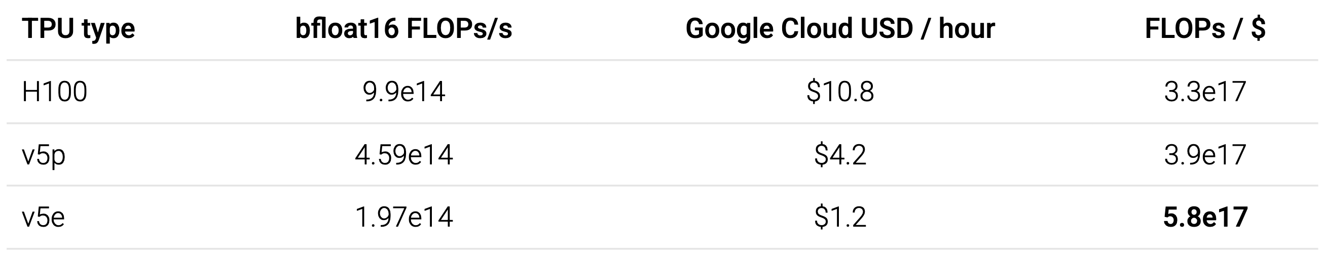
As a principle, FLOPs / $ is right. But the price for H100 GPUs is off by quite a lot. For instance, Modal offers serverless H100s (boot in <2s, premium offering) for $3.95/hr. A quick search shows you can get H100s for much cheaper than even that if you’re willing to run your own servers. Anyway, just take these prices with a grain of salt; the authors and GCP have a business incentive to make TPUs look good.

Some quick takeaways from this chapter:

• KV cache takes up a lot of space! Each token is about 1/440k the total size of the model in memory, assuming int8 quantization for both. If you have 32k context windows, this limits your batch size a lot. Quick-and-dirty explanation of the “440k” number is that it’s how much bigger the MLP params are.

• Consider doing int8 quantization but bf16 FLOPs. You don’t pay for the extra precision in FLOPs because batch size isn’t high enough to get to the point where matmul is compute-bound. Low-precision arithmetic may affect performance.

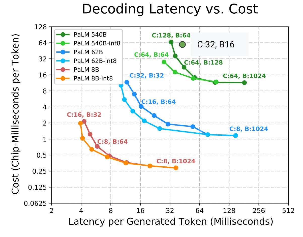
• You pay a lot for lower latency, below a point. These graphs are quite dramatic and show that if you have a very small batch size, you get to run super fast, but throughput sucks.

Part 9: How to Profile TPU Programs

We’ve finally started writing JAX. I really like JAX and so I’m familiar with the framework + its functional (even functorial?) style. But this is something new for me, using the JAX profiler, which is a tool for understanding TPU traces.

Review of the compiler pipeline: Jaxpr → StableHLO → HLO → TPU LLO. Or you can write custom kernels in Pallas.

The key thing to remember is that you can wrap code in jax.profiler.trace() contexts (as well as named scopes / calls) to generate linear traces, profiles, and XLA graph views that open in TensorBoard.

import jax

with jax.profiler.trace("/tmp/tensorboard"):
    key = jax.random.key(0)
    x = jax.random.normal(key, (1024, 1024))
    y = x @ x
    y.block_until_ready()

The visualization suite reminds me of pprof, which I guess makes sense as another Google product. Graphs, looking at the lowering of various parts of code, and a focus on the trace timeline first and foremost.

Profiling is never super fun, but general rules apply here. It becomes easier as you get fluent in the domain (e.g., author just happens to know “AllReduce + dynamic slice = ReduceScatter”), and it’s also definitely much more approachable if you come in with an idea of what you think the profile will look like and validate.

Part 10: Programming TPUs in JAX

There are three modes: fully automatic, explicit sharding (via type system), and manual sharding with shard_map().

It’s pretty cool to see these automatic sharding modes in JAX. All of the methods are pretty cutting-edge work. I first read about auto-sharding in 2022 via Alpa (OSDI ‘22), which also included inter-operator (pipeline) parallelism in its scope. Probably too much, but hey it was a research prototype.

Auto sharding mode:

1. You create a device mesh with jax.make_mesh(), with axis shapes and names. Each array gets a jax.NamedSharding set as its device on construction, which lets you specify how to shard the array across devices.

2. After that, jax.jit() allows you to specify in and out-shardings, and all intermediates are then automatically inferred (via heuristic) via Shardy (XLA).

3. You can then profile it. Maybe you see an issue, and give the compiler a hint with jax.lax.with_sharding_constraint() to change the behavior.

Explicit sharding mode:

1. You create a mesh as before but pass in the “Explicit” axis type.

2. Now, every array you create has sharding in its metadata / type. When you run an operation, it determines whether the sharding can be inferred cleanly or not. If it’s not possible to infer the best possible sharding, you have to resolve the ambiguity by providing an out_sharding kwarg.

Manual sharding mode with shard_map: (see also tutorial)

1. You write a program that runs on one device, in SPMD style like torch.

2. Decorate it with jax.shard_map(), and it will run on all devices in parallel with each device receiving a particular sharding.

3. Insert collective operations as needed like jax.lax.ppermute(), jax.lax.pmean(), jax.lax.all_gather(), etc.

Part 12: How to Think About GPUs

(Slightly out-of-order, leaving Part 11 until the end since it’s the conclusion.)

We have one last “addon” chapter, this one compares TPUs and GPUs. Their description of GPUs is short and witty.

A modern ML GPU (e.g. H100, B200) is basically a bunch of compute cores that specialize in matrix multiplication (called Streaming Multiprocessors or SMs) connected to a stick of fast memory (called HBM).

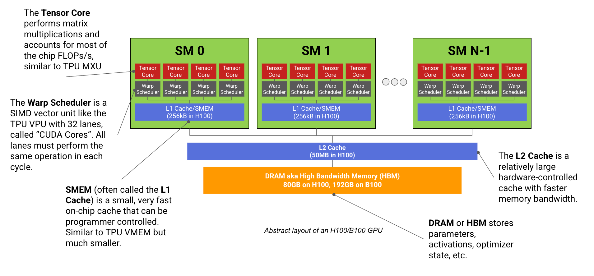
I’m pretty familiar with GPUs, having done some CUDA programming, so there’s a bunch of concepts here like warp = 32 threads, warp scheduler, divergence, shared memory, warpgroups (SM) and so on. GPUs are more general-purpose than TPUs, but they also have a huge chunk cut out for tensor cores that do matmul.

As I mentioned before, networking is very different in GPUs versus TPUs. Among nodes in a Scalable Unit (SU), GPUs get full bisection bandwidth, and every node is accessible to every other node by Infiniband switches in fat tree topology. You use RDMA to communicate.

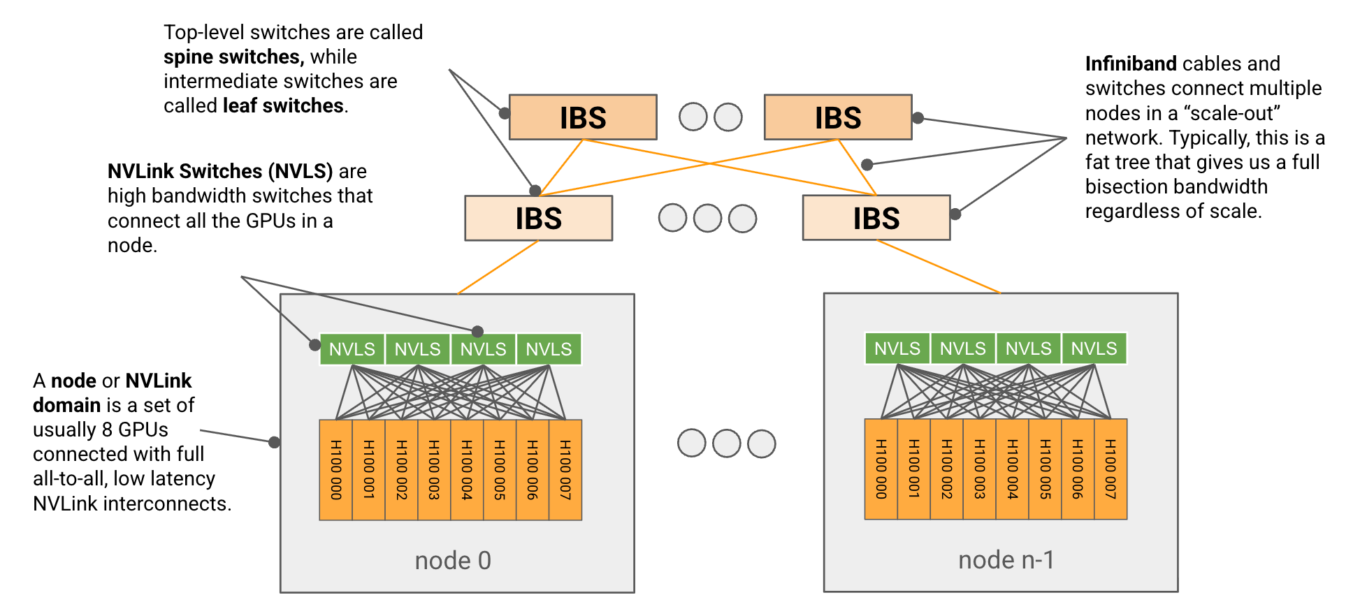
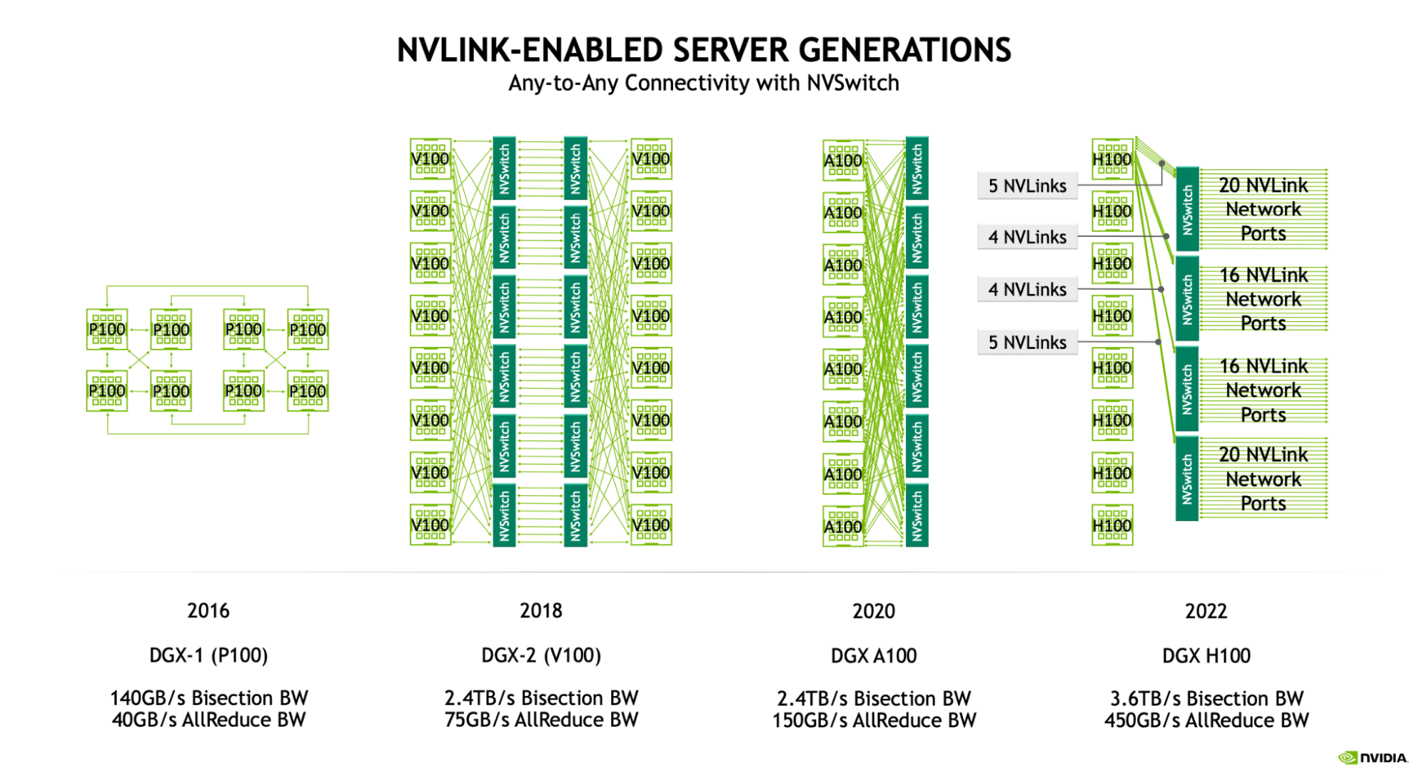
Each node itself has a few NVLink switches that offer very fast, 1-hop networking between its 8 GPUs, in an all-to-all fashion. This is a pretty nice diagram of how the connectivity changed over time!

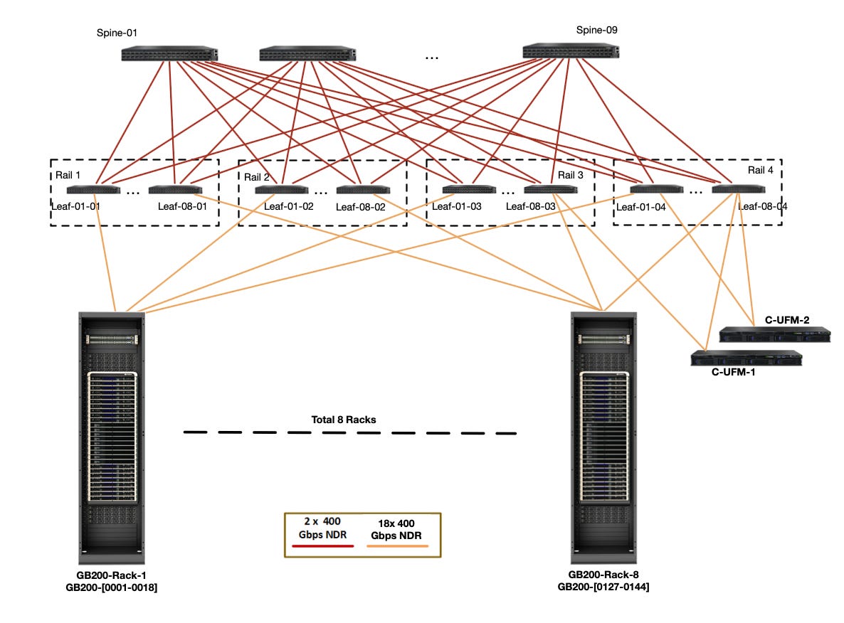
Beyond the level of a scalable unit, customers and cloud providers do various things to connect GPUs. It sounds like the most popular option is just Infiniband though. You need more high-bandwidth switches to support the fat tree as the number of GPUs and nodes grows. This may add to switching latency, but it also means that you get full connectivity, unlike TPUs.

Of course, everything changes with the “GB200 NVL72 SuperPod” system (what a name…). Instead of 8 devices on NVLink, you have 72. Great. Not going to think about that one for a while, haha.

The full connectivity changes up some collectives. AllReduce, ReduceScatter, and AllGather mostly stay the same, though latency can be reduced with an optimized implementation. AllToAll gets significantly faster because you can send the sharded data directly from one device to others.

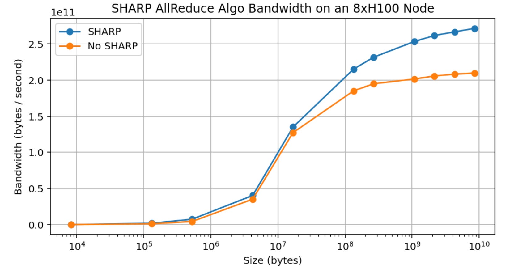
One fun gadget is SHARP, which lets you do reductions within the network switch itself. This theoretically reduces time by half, but the authors here only saw 30% improvement in practice. May slightly change up calculations!

The second half of the chapter follows with a bunch of lore on GPU training and inference, basically going through the same roofline calculations as before. It’s slightly different because you need to consider the inter-node bandwidth as well.

Remember that pipeline parallelism does not play well with FSDP due to the weight sharding getting screwed up by pipelines.

During training, you need a local batch size of about 2500 tokens per GPU. Besides that, you can combine model parallelism / expert parallelism (8-64 GPUs), then pipeline parallelism, and finally ZeRO-1 data parallelism.

Part 11: Conclusions and Further Reading

This was a great read. I’m happy that so many people came together to write this; the mental model and visual acuity are on point. Also a nice way to advertise TPUs (haha), at least in spreading awareness of their programming model.

It’s a “textbook” but definitely one of the more well-written textbooks I’ve seen, and it presents a nice calculus of sorts for reasoning about these systems. Kind of like a math book, where you introduce new complexity, help the reader get used to it, simplify and then move on to more difficult challenges.

I went through my notes again with a friend and realized that they’re quite sparse if you aren’t already familiar with parallelism. Sorry! Consider this a band-pass filter over the book’s content, made for Eric. :)